ABSTRACT: Public opinion survey responses regarding the desirability of changes in defense spending can be compressed into a single variable, the public opinion balance, which, when accompanied by a control variable measuring the proportion of responses in the “residuum” (no opinion or keep the status quo), permits an accurate prediction of subsequent changes in the rate of change of U.S. outlays from the mid-1960s through the 1980s. This finding cannot be interpreted as a simple case of “the public got what it wanted,” however, because public opinion was not autonomous or spontaneous, and defense decision makers themselves played a central role in shaping public opinion.
Introduction
Many analysts have tried to explain variations in U.S. defense spending. In a recent survey Robert E. Looney and Stephen L. Mehay (1990) listed nine types of variables believed to have had an influence. They also noted (p. 13) that “single theories have not been particularly accurate in . . . accounting for past spending patterns.” Their own econometric contribution, like those of many other analysts, proceeded on the assumption that domestic economic conditions and the Soviet threat were the important variables explaining changes in military spending. They remarked (p. 33) that several other possible causal factors, including public opinion, are not subject to empirical testing because of deficiencies in the data.
Notwithstanding Looney and Mehay’s observations, there is a substantial empirical literature in political science assessing the connection between public opinion and defense spending (Ostrom, 1978; Ostrom and Marra, 1986; Kriesberg and Klein, 1980; Russett, 1989, 1990; Russett and Graham, 1989; Hartley and Russett, 1992; and other studies cited in these sources). Although the political scientists who have studied public opinion have usually concluded that it has played a part in determining the size of the defense budget, they have not defined the public opinion variable operationally in a manner that exploits all the information contained in the responses to public opinion surveys. Some analysts have used as an operational variable either the percentage of poll respondents favoring increased defense spending or the percentage favoring decreased defense spending (Kriesberg and Klein, 1980, and Russett’s studies). Others have lost much of the information contained in the survey responses by transforming them into dichotomous variables (Ostrom, 1978; Ostrom and Marra, 1986).
The research findings we report here show that with a simple statistical model one can explain a high proportion of the variance of the annual rate of change of U.S. defense outlays from the mid-1960s through the 1980s. Public opinion can be measured in a way that exploits all the genuine information in the polls, and a single public opinion variable, with the several lags and a proper control, is the only one required for an accurate prediction of annual changes in defense outlays. When this statistical explanation is considered in the light of information about how the defense budget process operates, it suggests that defense spending was influenced by the effect of public opinion on both the executive branch and Congress. Notwithstanding the close relationship between public opinion and defense budget decision making, however, we argue that it would be unwarranted to conclude—à la simple democratic theory—that defense spending policy was simply a case in which “the public got what it wanted.”
Measuring Public Opinion
Political scientists and political sociologists have long employed public opinion survey data with sophistication to analyze attitudes, opinions, and ideologies (Bennett, 1980; McClosky and Zaller, 1984; Page and Shapiro, 1992). Defense economists occasionally cite such data (Stubbing, 1986, p. 13; Weida and Gertcher, 1987, p. 78), and one economist has attempted to use the data in estimating demand functions for defense (Hewitt, 1986, p. 480). We shall exploit public opinion data in a new way.
From various published sources and from data supplied to us by the Roper Center for Public Opinion Research and by researchers Thomas Graham and Thomas Hartley at Yale University, we have compiled a total of 193 comparable national surveys taken from 1949 to 1989 regarding opinion about defense spending.1 We have used the survey information only if the question put to the respondents allowed them the alternatives “spend more” and “spend less” and was specifically about spending, not about whether the armed forces should be enlarged, whether the nation’s defense is adequate, or other matters not explicitly about spending. Although the questions vary slightly in wording, we have used only those that seem identical in substance and devoid of cues that might bias the response (e.g., introductory statements referring to “the President’s plan” or calling attention to the federal deficit). Typical wording is: “There is much discussion as to the amount of money the government in Washington should spend for national defense and military purposes. How do you feel about this: do you think we are spending too little, too much, or about the right amount?” (Gallup poll, July 1969).
Altogether, 24 different polling organizations generated the evidence we analyze, although most of the data come from the large, well-known polling organizations (Gallup, Harris, Roper, NBC, CBS, ABC, and the National Opinion Research Center). All the polling organizations appear to use similar methods and produce results with similar degrees of sampling reliability, typically with standard deviations of about 2 percentage points. Between 1953 and 1965 there were several years without a survey asking a comparable question about defense spending. Because our statistical methods require a continuous series of data, we shall not analyze the pre-1965 data here. From 1965 onward there was at least one usable survey each year; after 1970 there were at least three per year and often ten or more. When multiple surveys are available, we have collapsed the results into a single number by simply averaging. Altogether, the time series on public opinion analyzed here contains information from 181 national surveys.
From the surveys, we have constructed a variable that compresses two responses into one. Our procedure creates an “opinion balance” variable (denoted OPBAL) by subtracting the percentage of respondents favoring less defense spending from the percentage favoring more. For example, if 30 percent of the respondents favor more and 20 percent favor less, the opinion balance has a value of +10. In this way we compress into a single variable all the survey response information related to the public’s preferences for a change in defense spending.
Notice, however, that the opinion balance variable alone does not capture all the information in the surveys potentially of interest to policy makers. Obviously, particular values of opinion balance can arise in many different ways (e.g., 20 - 10 = 10; 33 - 23 = 10; 51 - 41 = 10). Given a particular level of opinion balance, the “residuum” (denoted OPRES), which contains all those who either favor the existing level of spending or express no opinion, can be a greater or smaller percentage of all respondents. We do not think it serves any purpose to distinguish the two components of the residuum. Many of those who express a preference for the existing level of spending surely do so because they have little information or interest in the matter; hence in reality they do not differ from those who explicitly respond with “no opinion.”2 In any event, whether a respondent actively prefers the existing level of spending or has no opinion, the effect on policy decisions (if any) is the same—preservation of the status quo. However, the effect (if any) of a particular opinion balance can be presumed to vary with the size of the associated residuum: the greater the residuum, the smaller the effect of a given opinion (im)balance on spending decisions, because the residuum encourages policy makers to maintain the status quo.
In statistical models, one can deal with the problem of the residuum simply by including it as a variable along with the opinion balance variable in the regression equations. OPRES then serves as a control variable that allows one to interpret the effect of variations of OPBAL in a straightforward manner. OPRES itself has no a priori relation to the rate of change of defense spending; hence we advise against attempts to interpret the sign or statistical significance of its estimated regression coefficient.
What Happened?
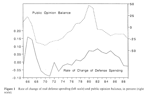
Figure 1 shows how the opinion balance (OPBAL) moved from 1965 to 1989. During the first three years of the Vietnam War the opinion balance remained positive, although it declined by 18 points between 1966 and 1967. The year 1968 witnessed the peak of U.S. engagement in the war as well as the Tet offensive, early in the year, that transformed many former supporters of the war into opponents (Russett and Graham, 1989, p. 252; Matusow, 1984, p. 391; Page and Shapiro, 1992, pp. 56-57, 232-234).3 In 1968 the opinion balance plummeted 38 points to reach -33. During the next two years it fell to even lower levels, with a trough of -39 in 1970. (Of course, given the sampling variance, changes of a few points cannot bear much weight.) After 1970 the opinion balance began to increase monotonically, slowly at first, then more rapidly during late 1970s. It first achieved a positive value (+7.5) in 1977. At its peak in 1980 the opinion balance stood at 46.7. It then fell for five years, with a huge drop of more than 45 percentage points in a single year, 1982—surely no statistical artifact.4 From 1986 to 1988 the balance remained virtually unchanged at about -15, roughly where it had been back in 1975, before falling another 10 points in 1989. Scanning the series, one gathers the distinct impression of cyclical change with a peak in 1966, a trough around 1970, steady increase toward another peak in 1980, then a quick decline to a low plateau in the second half of the 1980s.5
Figure 1. Rate of change of real defense spending (left scale) and public opinion balance, in percent (right scale).
Our defense spending variable is real national defense purchases of goods and services as measured in the national income and product accounts (U.S. Council of Economic Advisers, 1991, p. 287). This standard measure of defense spending, which is on a calendar-year basis, does not include military pensions, purchases of previously produced assets, or other transfer payments. Because the deflator constructed by the Commerce Department for defense expenditures is problematic in several respects (Weida and Gertcher, 1987, p. 63; Smith, 1989, pp. 350-51), we used the GNP deflator to reduce the nominal spending figures to constant 1982 dollars (U.S. Council of Economic Advisers, 1991, p. 290). This deflator is actually more appropriate in any event if one thinks of defense spending in terms of its societal opportunity costs, that is, as necessarily entailing sacrifices of generalized national product.
In part because the level of real defense spending was highly autocorrelated during the years under investigation (r = 0.91 for the one-year lag, r = .76 for the two-year lag), for statistical modeling we employ a transformation, namely, the annual proportional rate of change (denoted OUTLAY GROWTH). Employing this transformation also makes sense theoretically, as it allows us to examine empirically the exact relation at issue, that is, the relation between the intensity of the public’s preference for change in defense spending and the actual rate of change.
The OUTLAY GROWTH series, shown in Figure 1, also gives one an impression of cyclical movement, although the pattern is not quite so smooth as that of the opinion balance. After reaching the Vietnam War peak in calendar year 1968, real military outlays began to fall. During the next eight years the annual rate of change varied but remained negative in every year. (Note that the small local growth-rate peak at 1972 was at least partly spurious, reflecting the stringent price controls in effect throughout the year, which caused the reported GNP deflator to rise by less than the actual rate of inflation, much of which was concealed in 1972 then revealed in 1973. Correction of the data for this mismeasurement, which is beyond the scope of the present paper, would produce a smoother change of our series between 1971 and 1974.) Between 1973 and 1982 OUTLAY GROWTH rose haltingly but substantially, reaching a peak of 8.4 percent in 1982. It then diminished, finally becoming negative in 1988 and 1989.
Scanning Figure 1, one suspects that the two series might have some relation. During the period 1969-1976 the opinion balance was always negative, as was the annual change of real defense spending. In 1977, when the opinion balance first became positive again, real defense spending increased for the first time since 1968. In 1979 and 1980 both series increased, and in the latter year the opinion balance reached a maximum. After 1981, however, the opinion balance plummeted, becoming negative again in 1982. The rate of change of defense outlays did not begin its descent until after 1982 and did not become negative until 1988. All in all, there seems to be a connection here, but without a more systematic analysis one has no way to know whether a causal relation existed and, if so, in which direction it ran.
Predictive Antecedence
An obvious statistical technique for examining these questions is Granger causality testing (Freeman, 1983; Kinsella, 1990). Although econometricians have concluded that this technique alone cannot establish the presence of causality in the substantive sense—that is, exogeneity in a structural model (Leamer as quoted in Baek, 1991, p. 252)—it can be used to refute claims of exogeneity. To apply a formula stated by Thomas Sargent to the present case, there will exist an equation expressing OUTLAY GROWTH as a one-sided distributed lag of OPBAL with OPBAL strictly exogenous if and only if OUTLAY GROWTH fails to Granger cause OPBAL (Sargent as quoted in Freeman, 1983, p. 329). So, the absence of Granger causation tells us something, while the presence of Granger causation is merely suggestive. Following David Kinsella (1990, p. 300), we employ Granger causality testing only as “an appropriate first step in structural modeling . . . when theoretically-derived restrictions are lacking or when equally persuasive but opposing causal arguments need assessing.” (John Freeman [1983, p. 329]) also views Granger causality testing as only a useful first step in model building.) If the Granger test indicates predictive antecedence in one direction but not the other, then further testing is appropriate, with the postulated exogeneity as indicated by the Granger causality tests.
Contributors to the literature have considered the possibility that the causal relation between public opinion and defense spending might run in either direction (Russett and Graham, 1989, pp. 241-243; Hartley and Russett, 1992). To test for Granger causality running from opinion to spending, we estimated the parameters of an equation in which the rate of change of defense outlays (OUTLAY GROWTH) was regressed on itself lagged once, twice, thrice, and four times as well as on correspondingly lagged OPBAL and OPRES.6 We then tested the hypothesis that the coefficients of lagged OPBAL are jointly zero—that is, there is no Granter causation running from opinion to the growth rate of spending. We also performed a similar test for Granger causality running from the rate of change of defense spending to the public opinion balance. This test differs in the number of lags employed.7 The estimated equation also includes the contemporaneous value of OUTLAY GROWTH as well as lagged values.8
The two tests yielded different results. In the equation estimated to identify Granger causality running from the rate of change of defense spending to the public opinion balance, the null hypothesis—no Granger causality—cannot be rejected at any customary level of Type I error (F[2,15] = 2.14; p = 0.151). In contrast, the result of the test for Granger causality running from the opinion balance to the rate of growth of defense spending is consistent with rejection of the null hypothesis at a level of Type I error just over 8 percent (F[4.8] = 3.07; p = 0.083).
Employing Sargent’s formula again, we conclude from these tests that there probably does exist an equation expressing OUTLAY GROWTH as a one-sided distributed lag of OPBAL with OPBAL strictly exogenous, because the test results indicate that OUTLAY GROWTH probably did not Granger cause OPBAL but—at a fairly high level of confidence—OPBAL did Granger cause OUTLAY GROWTH. Beyond this limited conclusion, however, Granger causality testing cannot take us.
Table 1. Regression estimates of the relation between the rate of change
of real defense spending and the public opinion balance, 1965-1989
| Variable | Equation 1 | Equation 2 | Equation 3 |
| CONSTANT | -0.0743 | -0.0474 | 0.0620 |
| (-1.4285) | (-0.8490) | (0.8042) | |
| OPBAL(-1) | 0.0023 | 0.0011 | |
| (6.1895) | (2.5592) | ||
| OPBAL(-2) | 0.0018 | 0.0013 | |
| (4.6229) | (2.1171) | ||
| OPBAL(-3) | -0.0002 | ||
| (-0.3877) | |||
| OPBAL(-4) | 0.0003 | ||
| (0.6683) | |||
| OPRES(-1) | 0.0024 | 0.0008 | |
| (2.0934) | (0.8812) | ||
| OPRES(-2) | 0.0016 | 0.0009 | |
| (1.2815) | (1.1234) | ||
| OPRES(-3) | 0.0010 | ||
| (1.1097) | |||
| OPRES(-4) | -0.0035 | ||
| (-4.4165) | |||
| R2 | 0.649 | 0.518 | 0.889 |
| Adjusted R2 | 0.616 | 0.470 | 0.815 |
| SEE | 0.040 | 0.042 | 0.023 |
| D-W | 1.204 | 1.514 | 1.554 |
| F | 19.447 | 10.471 | 11.997 |
| Years Predicted | 66-89 | 67-89 | 69-89 |
Note: For variables OPBAL(i) and OPRES(i), i is the number of years the variable
is lagged. Parenthetical numbers beneath the regression coefficients are Student’s t statistics.
The Structure of Causation
Because of the nature of the hypothesis tests associated with the Granger technique (i.e., tests that the coefficients are jointly zero), one cannot identify which lagged value of OPBAL might have been associated, and how much, with changes in the rate of change of real defense spending. To answer these questions, we have estimated several variants of equations in which the dependent variable is OUTLAY GROWTH and the explanatory variable is OPBAL with one or more lags (and each OPBAL with its corresponding lagged OPRES). Three of these estimated equations appear in Table 1.9
The most remarkable aspect of the results is that these simple equations explain a high proportion of the variance of the dependent variable.10 Using only OPBAL(-1)—that is, one-year-lagged OPBAL (along with the corresponding OPRES)—one accounts for 65 percent of the variance. Using just OPBAL(-2) instead (along with the corresponding OPRES), one obtains a somewhat lower R2 but still explains more than half the variance. With four lags of OPBAL entered simultaneously (along with corresponding OPRES variables), one can account for a high proportion of the variance (R2= 0.89). To achieve such a high degree of statistical explanation of the rate of change of defense spending by using only a single explanatory variable (along with its control) is extraordinary. After all, analysts have attributed changes in defense spending to a large number of variables (Looney and Mehay, 1990; Schneider, 1988). Although our findings by themselves do not necessarily refute any claims regarding the causality of other variables, they demonstrate that one can with considerable precision account for changes in defense spending from the mid-1960s through the 1980s with reference to public opinion data alone. What are we to make of this remarkable finding?
Interpretation
Defense spending in a particular year is the final outcome of a sequence of actions by various institutionally situated actors who act with greater or lesser influence at various stages of the budget process. The actual change in defense outlays from calendar year t-1 to calendar year t reflects mainly the appropriations legislation enacted by Congress late in calendar year t-1, which sets expenditures for fiscal year t. The detailed budget proposals presented to Congress by the President in January of year t-1 were composed within the executive branch during the course of year t-2. Even earlier, armed forces personnel were making plans with an eye to the future budgetary requirements of research and development for new weapons systems, procurement of existing weapons, changes in force levels and troop deployments, and many other aspects of managing the military establishment.11
Our findings indicate that public opinion in both years t-1 and t-2 affected, more or less equally, the rate of change of real defense outlays in year t. This finding would seem to show that public opinion influenced both the executive branch, as it composed its future budget requests during year t-2, and Congress, as it reacted to the proposals, generally cutting the requested amount of funding to some extent during year t-1. But one ought to be skeptical of such a simple view of the process. The mere fact of congressional cuts of presidential requests during year t-1, for example, is insufficient to establish that the estimated effect of public opinion during that year reflects solely a congressional response to public preferences at that time. Nor is the existence of a two-year-lagged effect necessarily indicative of nothing more than an executive branch response to public preferences at that time (t-2).
At no time were decisions by one branch of government independent of what was being sought by the other. In reality the executive branch normally entered into a political arrangement with Congress whereby each side could better achieve its important aims. The armed forces got the resources they wanted most urgently, and Congress got political credit for slashing a “bloated” defense request. Building “cut insurance” into the President’s request was the key to this deal. As described by Richard Stubbing (1986, pp. 96-97), a veteran defense analyst for the Office of Management and Budget, the process worked as follows:
each year the executive branch anticipates the congressional need to lower defense spending and therefore includes in its request extra funds for removal by the Congress. . . . [I]n the back rooms DoD and congressional staff are working out mutually acceptable lists of reductions which will cause little or no damage to the program DoD really wants to pursue. These “cut insurance” funds can then be slashed from the defense-budget request by the Congress, permitting members to demonstrate their fiscal toughness to their constituents without harming the defense program. Almost all the so-called “cuts” are simply deferred to the next year’s budget, and the overall total is never cut below the minimum level acceptable to the military leadership.
Similarly the President’s proposal normally omits or underfunds certain items (e.g., equipment for the reserves and national guard). The executive branch makes its proposals with full awareness that Congress will “add on” funding for these items and then take political credit for the supplements with the ostensibly favored constituents.
It would be unwarranted, however, to interpret our findings simply as follows. Indirectly the mass public decides how the defense budget will be changed, by expressing its preferences to the pollsters. The executive branch, with some preliminary congressional input and provision for “cut insurance,” responds to the polls as it crafts the proposals it will present to Congress the following January. Afterward both Congress and the executive branch, jointly responding to the more recent polls, make the mutual (and partly spurious) adjustments that immediately precede the autumn enactment of appropriations legislation. This view, though an improvement over the usual depiction, is nonetheless still unacceptable, because it takes the public’s opinions themselves to be autonomous or spontaneous.
Such autonomy is implausible. In the extreme opposite case, as described by Russett and Graham (1989, p. 257), “policymakers might first form a new opinion and then persuade opinion leaders in the media, who in turn persuade the mass public so that, finally, the very people in government who initiated the change can then ‘respond’ to public opinion.”12 In countless ways the President and other leading political figures, including those in charge at the Pentagon, try to sway public opinion. One may argue about the extent to which, and the conditions under which, they succeed in molding public opinion. There is substantial evidence, however, that their efforts often have some effect (Ginsberg, 1986; Page and Shapiro, 1992). Hence one cannot view public opinion as independent of the desires of the very officials toward whom the public’s preferences for governmental actions are directed.
Although surprising at first, the finding that public opinion alone is a powerful predictor of changes in defense spending seems, upon reflection, exactly what one ought to have expected. Despite how defense (and other) analysts normally conceive of public opinion—as one element in a long list of commensurable influences (Looney and Mehay, 1990; Schneider, 1988)—public opinion actually stands conceptually on a plane by itself. It is a different kind of variable. Public opinion expresses people’s preferences regarding policy action. Other “causes” normally advanced by analysts (domestic economic conditions, perceived foreign threats, and so forth) do not directly determine changes of defense spending; rather, they determine what decision makers and the public prefer with regard to changes of defense spending. Once public opinion has revealed itself in the polls (or in other ways), government officials, especially those immediately concerned with reelection, face a constraint. They must either act in accordance with public opinion or bear the political risk inherent in deviating form it.
There is, however, a way to loosen the constraint. Politicians who, for whatever reason, do not want to act in accordance with public opinion can argue their case. They can try to mold as well as merely react to public opinion. Clearly a contest for the determination of public opinion goes on ceaselessly, becoming especially active or noticeable from time to time. This contest is at the very heart of the political process. Although certain facts, such as the government deficit or the rate of inflation, cannot be denied, many other “facts,” such as the detailed military capabilities and intentions of potential adversaries, are known—if indeed they are known at all—only to members of the national security elite.13 Given their capacity to control access to important information, defense leaders and insiders have disproportionate ability to mold public opinion. They can also exploit their positions of authority to try to change the meaning or weight the public attaches to known, indisputable facts. Clearly, however, their power is far from absolute, as shown the large fluctuations of public opinion and particularly its movement at times in a direction obviously disfavored by the national security elite.14
Once public opinion has been deflected as much as possible by defense policy makers, whether in Congress or the executive branch, they have substantial incentives to match their defense spending decisions more or less closely with the public’s ultimate preference—hence the close association reported here. We emphasize, however, that important aspects of the defense budget process are (1) the status of public opinion as a single proximate cause incorporating and expressing a variety of more remote determinants of spending decisions and (2) the ceaseless contest among rival interests, within as well as outside the government, to move public opinion in a desired direction.
Conclusion
Public opinion survey responses regarding the desirability of changes in defense spending can be compressed into a single variable, the public opinion balance, which, when accompanied by a control variable measuring the proportion of responses in the “residuum” (no opinion or keep the status quo), permits an accurate prediction of subsequent changes in the rate of change of defense outlays from the mid-1960s through the 1980s. In a model with four lags of OPBAL, 89 percent of the variance in OUTLAY GORWTH can be statistically explained. Public opinion lagged one year and public opinion lagged two years had roughly the same influence.
One is not justified, however, in regarding public opinion as entirely autonomous or spontaneous. There occurs a ceaseless contest over the determination of public opinion, and in this contest defense policy makers, whose preferences may differ from those of the mass public, occupy a powerful position. Hence, even after finding a strong association between OUTLAY GROWTH and lagged OPBAL, we remain uncertain of the extent to which public opinion about defense spending was independent of the desires of government officials and hence may be viewed as an important autonomous determinant of spending decisions. Future modelers and interpreters of defense spending would do well to take into account this more complex and realistic view of defense budget policymaking.
Footnotes:
*We thank Bruce Russett, Thomas Hartley, and Thomas Graham for providing us with unpublished material, Josh Gotkin for valuable research assistance, and four referees for corrections and suggestions.
1. The authors will provide upon request a list of the raw data and their sources.
2. Bishop (1987, p. 229) reports that a status quo option “usually attract[s] a substantial number of people who may be ambivalent about the other alternatives presented to them.” Hartley and Russett (1992, p. 907) remark that “with the problem conceptualized in terms of change, those with no current interest could either fail to express an opinion or simply support the status quo.”
3. Page and Shapiro (1992, p. 233) describe the “Tet-induced drop in the proportion of hawks” as “one of the largest, most abrupt opinion changes” ever measured by opinion surveys.
4. Inspection of the individual surveys shows that the collapse of the opinion balance began well before the end of 1981. Unfortunately, seven of the nine usable polls in 1981 took place during the first four months of the year.
5. The appendix gives the complete series for OPBAL and OPRES.
6. For OUTLAY GROWTH four lags are optimal in that they minimize Akaike’s Final Prediction Error (FPE) criterion. Given four lags of OUTLAY GROWTH, Akaike’s FPE tends to decline as more lags of OPBAL and OPRES are employed up to six lags. We cannot use so many lags, however, given our small sample size and the consequent scarcity of degrees of freedom. Four lags of OPBAL and OPRES is a reasonable compromise.
7. For OPBAL and OPRES, Akaike’s FPE is minimized by the use of two lags. Given two lags of OPBAL and OPRES, the use of one lag of OUTLAY GROWTH minimizes the FPE.
8. Conceivably, the current rate of change of defense outlays could influence current public opinion concerning the desired rate of change of defense outlays. However, it is quite unlikely that the current public opinion balance could affect the current rate of change of defense outlays, because the latter has been largely predetermined by policy makers during previous years.
9. To test the sensitivity of the estimates to the sample period 1965-1989, each of the equations in Table 1 was estimated for a sample period without the first three years (i.e., 1968-1989) and for a sample period without the last three years (i.e., 1965-1986). The results are essentially the same as those reported in Table 1.
10. Because the correlogram of autocorelations and partial autocorrelations suggests the possibility of a first-order autoregressive error, we also made estimates using the Cochran-Orcutt technique. The results are broadly similar to the OLS results in Table 1.
11. For recent description and analysis of the defense budget process, see Stubbing, 1986, pp. 55-105, and Weida and Gertcher, 1987, pp. 10-14, 56-61.
12. For an extended argument that something akin to this has become the rule rather than the exception in the politics of modern liberal democracies, see Ginsberg, 1986.
13. Especially was this so during the Cold War era, when the Soviet Union was an isolated, tightly controlled society with a very secretive government.
14. For example, in 1987 Secretary of Defense Caspar Weinberger complained that “new weapons can be developed by our adversaries ... much more rapidly because [in the USSR] there are no funding restraints imposed by public opinion.” Weinberger, 1987, p. 16. For extended discussion of the molding of public opinion by the authorities and the limits of such actions, see Page and Shapiro, 1992.
References:
Baek, E. G. (1991) Defence spending and economic performance in the United States: Some structural VAR evidence. Defence Economics 2 (3), 251-264.
Bennett, W. L. (1980) Public Opinion in American Politics. New York: Harcourt Brace Jovanovich.
Bishop, G. F. (1987) Experiments with the middle response alternative in survey questions. Public Opinion Quarterly, 51 (2), 220-232.
Freeman, J. R. (1983) Granger causality and the time series analysis of political relationships. American Journal of Political Science, 27 (2), 327-358.
Ginsberg, B. (1986) The Captive Public: How Mass Opinion Promotes State Power. New York: Basic Books.
Hartley, T. and Russett, B. (1992) Public opinion and the common defense: Who governs military spending in the United States? American Political Science Review, 86(4), 905-915.
Hewitt, D. (1986) Fiscal illusion from grants and the level of state and federal expenditures. National Tax Journal, 39 (4), 471-483.
Kinsella, D. (1990) Defence spending and economic performance in the United States: A causal analysis. Defence Economics, 1 (4), 295-309.
Kriesberg, L. and Klein, R. (1980) Changes in public support for U.S. military spending. Journal of Conflict Resolution, 24 (1), 79-111.
Looney, R. E. and Mehay, S. L. (1990) United States defence expenditures: trends and analysis. In The Economics of Defence Spending: An International Survey, edited by K. Hartley and T. Sandler, pp. 13-40. London: Routledge.
Matusow, A. J. (1984) The Unraveling of America: A History of Liberalism in the 1960s. New York: Harper & Row.
McClosky, H. and Zaller, J. (1984) The American Ethos: Public Attitudes toward Capitalism and Democracy. Cambridge, Mass.: Harvard University Press.
Ostrom, C. W., Jr. (1978) A reactive linkage model of the U.S. defense expenditure policymaking process. American Political Science Review, 72 (3), 941-957.
Ostrom, C. W., Jr. and Marra, R. F. (1986) U.S. defense spending and the Soviet estimate. American Political Science Review, 80 (3), 819-842.
Page, B. I. and Shapiro, R. Y. (1992) The Rational Public: Fifty Years of Trends in Americans’ Policy Preferences. Chicago: University of Chicago Press.
Russett, B. (1989) Democracy, public opinion, and nuclear weapons. In Behavior, Society, and Nuclear War, edited by P. Tetlock et al., pp. 174-208. New York: Oxford University Press.
Russett, B. (1990) Controlling the Sword: The Democratic Governance of National Security. Cambridge, Mass.: Harvard University Press.
Russett, B. and Graham, T. W. (1989) Public opinion and national security policy: Relationships and impacts. In Handbook of War Studies, edited by M. I. Midlarsky, pp. 239-257. Boston: Unwin Hyman.
Schneider, E. (1988) Causal factors in variations in US postwar defense spending, Defense Analysis, 4 (1), 53-79.
Smith, R. P. (1989) Models of military expenditure. Journal of Applied Econometrics, 4 (4), 345-359.
Stubbing, R. A. (1986) The Defense Game: An Insider Explores the Astonishing Realities of Americas Defense Establishment. New York: Harper & Row.
U.S. Council of Economic Advisers (1991) Annual Report. Washington, DC: U.S. Government Printing Office.
Weida, W. J. and Gertcher, F. L. (1987) The Political Economy of National Defense. Boulder: Westview Press.
Weinberger, C. W. (1987) Report of the Secretary of Defense Casper W. Weinberger to the Congress. Washington, DC: U.S. Government Printing Office.
Appendix: Indexes of Opinion Balance and the Residuum
| Year | OPBAL | OPRES | Year | OPBAL | OPRES | |
| 1965 | 12.00 | 56.00 | 1978 | 8.71 | 48.43 | |
| 1966 | 23.00 | 51.00 | 1979 | 19.40 | 40.20 | |
| 1967 | 5.00 | 51.00 | 1980 | 46.69 | 27.31 | |
| 1968 | -33.00 | 27.00 | 1981 | 40.45 | 30.89 | |
| 1969 | -35.00 | 44.34 | 1982 | -5.07 | 45.89 | |
| 1970 | -39.00 | 41.00 | 1983 | -5.33 | 40.93 | |
| 1971 | -32.50 | 44.00 | 1984 | -11.90 | 46.30 | |
| 1972 | -29.34 | 50.00 | 1985 | -18.46 | 46.20 | |
| 1973 | -27.80 | 48.20 | 1986 | -14.50 | 44.22 | |
| 1974 | -22.85 | 48.57 | 1987 | -15.06 | 45.94 | |
| 1975 | -12.33 | 46.33 | 1988 | -14.70 | 52.50 | |
| 1976 | -7.00 | 47.28 | 1989 | -25.09 | 47.27 | |
| 1977 | 7.50 | 49.50 | ||||